Checking Airborne Radar Echo Sounding data#
Author: Alice Fremand (@almand) & Julien Bodart (@julbod)
Date: 12/11/2021
Aim#
The goal of this tutorial is to easily check radar echo sounding data from either NetCDF or SEG-Y formatted files.
Virtual environment#
For the code to run, it is important to install the correct dependancies and libraries. In particular the following libraries are crucial for the code to run:
netCDF4 module to check NetCDF data in python
obspy module to check SEGY data in python
To set up the virtual environment with Conda:#
>conda create -n aerogeophysics_env
>conda activate aerogeophysics_env
>conda config --env --add channels conda-forge
>conda config --env --set channel_priority strict
>conda install python=3 obspy
>conda install netCDF4
To set up the virtual environment on UNIX:#
Load your python module:
module load python/conda3
Then in the folder where you have your code, you need to launch:
python3 -m venv aerogeophysics_env
It will create a folder with all the environment for python. To activate the virtual environment you need to lauch it:
source aerogeophysics_env/bin/activate.csh
You need to make sure that [aerogeophysics_env] appears before your name on the machine. That means that you are using the virtual environment Then you need to upgrade pip which is the command that install the packages
python3 -m pip install --upgrade pip
And install the other libraries
python3 -m pip install obspy
In this tutorial, the virtual environment is already set up. The list of the current libraries loaded is given in the list below.
pip list
Package                       Version
----------------------------- -------------------
affine                        2.3.0
alabaster                     0.7.12
anyio                         3.3.3
appdirs                       1.4.4
argh                          0.26.2
argon2-cffi                   21.1.0
arrow                         1.1.0
astroid                       2.5.8
async-generator               1.10
atomicwrites                  1.4.0
attrs                         21.2.0
autopep8                      1.5.6
Babel                         2.9.1
backcall                      0.2.0
backports.functools-lru-cache 1.6.4
bcrypt                        3.2.0
beautifulsoup4                4.9.3
binaryornot                   0.4.4
black                         21.5b2
bleach                        3.3.0
brotlipy                      0.7.0
cached-property               1.5.2
certifi                       2021.5.30
cffi                          1.14.5
cftime                        1.5.0
chardet                       4.0.0
click                         7.1.2
click-plugins                 1.1.1
cligj                         0.7.2
cloudpickle                   1.6.0
colorama                      0.4.4
cookiecutter                  1.7.0
cryptography                  3.4.7
cycler                        0.10.0
decorator                     4.4.2
defusedxml                    0.7.1
diff-match-patch              20200713
docutils                      0.17.1
entrypoints                   0.3
et-xmlfile                    1.1.0
Fiona                         1.8.18
flake8                        3.8.4
future                        0.18.2
GDAL                          3.1.4
geopandas                     0.9.0
greenlet                      1.1.0
h5py                          3.2.1
idna                          2.10
imageio                       2.9.0
imagesize                     1.2.0
importlib-metadata            4.5.0
inflection                    0.5.1
intervaltree                  3.0.2
ipykernel                     5.5.5
ipython                       7.24.1
ipython-genutils              0.2.0
isort                         5.8.0
jedi                          0.17.2
Jinja2                        3.0.1
jinja2-time                   0.2.0
joblib                        1.0.1
json5                         0.9.6
jsonschema                    3.2.0
jupyter-client                6.1.12
jupyter-core                  4.7.1
jupyter-server                1.11.1
jupyterlab                    3.1.18
jupyterlab-pygments           0.1.2
jupyterlab-server             2.8.2
keyring                       23.0.1
kiwisolver                    1.3.1
lazy-object-proxy             1.6.0
lxml                          4.6.3
mapclassify                   2.4.2
MarkupSafe                    2.0.1
matplotlib                    3.4.2
matplotlib-inline             0.1.2
mccabe                        0.6.1
mistune                       0.8.4
mplcursors                    0.4
munch                         2.5.0
mypy-extensions               0.4.3
nbclassic                     0.3.2
nbclient                      0.5.3
nbconvert                     6.0.7
nbformat                      5.1.3
nest-asyncio                  1.5.1
netCDF4                       1.5.6
networkx                      2.5.1
notebook                      6.4.4
numpy                         1.20.3
numpydoc                      1.1.0
obspy                         1.2.2
olefile                       0.46
openpyxl                      3.0.9
OWSLib                        0.24.1
packaging                     20.9
pandas                        1.2.4
pandocfilters                 1.4.2
paramiko                      2.7.2
parso                         0.7.0
pathspec                      0.8.1
pdc-di                        0.20
pexpect                       4.8.0
pickleshare                   0.7.5
Pillow                        8.2.0
pip                           21.1.2
pluggy                        0.13.1
poyo                          0.5.0
prometheus-client             0.11.0
prompt-toolkit                3.0.18
psutil                        5.8.0
ptyprocess                    0.7.0
pycodestyle                   2.6.0
pycparser                     2.20
pydocstyle                    6.1.1
pyflakes                      2.2.0
Pygments                      2.9.0
pylint                        2.8.2
pyls-black                    0.4.6
pyls-spyder                   0.3.2
PyNaCl                        1.4.0
pyOpenSSL                     20.0.1
pyparsing                     2.4.7
pyproj                        3.1.0
PyQt5                         5.12.3
PyQt5-sip                     4.19.18
PyQtChart                     5.12
PyQtWebEngine                 5.12.1
pyreadline                    2.1
pyrsistent                    0.17.3
pyshp                         2.1.3
PySocks                       1.7.1
python-dateutil               2.8.1
python-jsonrpc-server         0.4.0
python-language-server        0.36.2
pytz                          2021.1
pywin32                       300
pywin32-ctypes                0.2.0
pywinpty                      1.1.4
PyYAML                        5.4.1
pyzmq                         22.1.0
QDarkStyle                    3.0.2
qstylizer                     0.2.0
QtAwesome                     1.0.2
qtconsole                     5.1.0
QtPy                          1.9.0
rasterio                      1.2.1
regex                         2021.4.4
requests                      2.25.1
requests-unixsocket           0.2.0
rope                          0.19.0
Rtree                         0.9.7
scikit-learn                  0.24.2
scipy                         1.6.3
segyio                        1.9.3Note: you may need to restart the kernel to use updated packages.

Send2Trash                    1.8.0
setuptools                    49.6.0.post20210108
Shapely                       1.7.1
six                           1.16.0
sniffio                       1.2.0
snowballstemmer               2.1.0
snuggs                        1.4.7
sortedcontainers              2.4.0
soupsieve                     2.0.1
Sphinx                        4.0.2
sphinxcontrib-applehelp       1.0.2
sphinxcontrib-devhelp         1.0.2
sphinxcontrib-htmlhelp        2.0.0
sphinxcontrib-jsmath          1.0.1
sphinxcontrib-qthelp          1.0.3
sphinxcontrib-serializinghtml 1.1.5
spyder                        5.0.4
spyder-kernels                2.0.4
SQLAlchemy                    1.4.18
terminado                     0.12.1
testpath                      0.5.0
textdistance                  4.2.1
threadpoolctl                 2.1.0
three-merge                   0.1.1
tinycss2                      1.1.0
toml                          0.10.2
tornado                       6.1
traitlets                     5.0.5
typed-ast                     1.4.3
typing-extensions             3.10.0.0
ujson                         4.0.2
urllib3                       1.26.5
watchdog                      2.1.2
wcwidth                       0.2.5
webencodings                  0.5.1
websocket-client              1.2.1
wheel                         0.36.2
whichcraft                    0.6.1
win-inet-pton                 1.1.0
wincertstore                  0.2
wrapt                         1.12.1
xlrd                          2.0.1
yapf                          0.31.0
zipp                          3.4.1
Load the relevant modules#
import netCDF4 as nc
from obspy.io.segy.segy import _read_segy
import matplotlib.pyplot as plt
import matplotlib.ticker as ticker
from matplotlib import transforms
import numpy as np
Check the NetCDF files#
Example given for GRADES-IMAGE data.
Data available for download here: Corr, H. (2021). Processed airborne radio-echo sounding data from the GRADES-IMAGE survey covering the Evans and Rutford Ice Streams, and ice rises in the Ronne Ice Shelf, West Antarctica (2006/2007) (Version 1.0) [Data set]. NERC EDS UK Polar Data Centre. https://doi.org/10.5285/C7EA5697-87E3-4529-A0DD-089A2ED638FB
Read the NetCDF#
f=nc.Dataset('D:/British_Antarctic_Survey/data/GRADES_IMAGE_0607/netcdf/GRADES_IMAGE_G06.nc', 'r')
Check the metadata information#
By printing f, we can read the metadata and obtain information about the variables and their respective dimensions
print(f.ncattrs())
['title', 'summary', 'history', 'keywords', 'Conventions', 'standard_name_vocabulary', 'acknowlegement', 'institution', 'license', 'location', 'instrument', 'platform', 'source', 'time_coverage_start', 'time_coverage_end', 'flight', 'campaign', 'creator_name', 'geospatial_lat_min', 'geospatial_lat_max', 'geospatial_lon_min', 'geospatial_lon_max', 'radar_parameters', 'antenna', 'digitiser', 'processing', 'resolution', 'GPS', 'projection', 'references', 'metadata_link', 'related_datasets', 'publisher_name', 'publisher_type', 'publisher_email', 'publisher_link', 'comment']
print(f)
<class 'netCDF4._netCDF4.Dataset'>
root group (NETCDF4 data model, file format HDF5):
    title: Processed airborne radio-echo sounding data from the GRADES-IMAGE survey covering the Evans and Rutford Ice Streams, and ice rises in the Ronne Ice Shelf, West Antarctica (2006/2007)
    summary: An airborne radar survey was flown as part of the GRADES-IMAGE project funded by BAS over the Antarctic Peninsula, Ellsworth Mountains and Filchner-Ronne Ice Shelf
    (also including the Evans Ice stream and Carson Inlet) mainly to image englacial layers and bedrock topography during the 2006/07 field season.
    Operating from temporary field camps at Sky Blu, Partiot Hills and out of RABID depot (Rutford Ice Stream), we collected ~27,550 km of airborne radio-echo sounding data over 100 hours of surveying.
    Our aircraft was equipped with dual-frequency carrier-phase GPS for navigation, radar altimeter for surface mapping, wing-tip magnetometers, and a new ice-sounding radar system (PASIN).
    Note that there was no gravimetric element to this survey.

    We present here the full radar dataset consisting of the deep-sounding chirp and shallow-sounding pulse-acquired data in their processed form, as well as the navigational information of each trace,
    the surface and bed elevation picks, ice thickness, and calculated absolute surface and bed elevations.
    The radar data provided in this NetCDF is also provided separately as georeferenced SEGY files for import into seismic-interpretation software.

    Details of survey location and design are presentend in Jeoffry et al. 2018 (ESSD, 10,711-725).
    More information on the radar system and processing can be found in Corr et al. 2007 (Terra Antartica Reports, 13, 55-63).
    history: This NetCDF contains the deep-sounding chirp and shallow-sounding pulse-acquired data (see the 'radar_parameters' attribute below) in the following structure:
    'chirp_data': Radar data for the processed (coherent) chirp
    'pulse_data': Radar data for the processed (incoherent) pulse

    Both radar variables have the same length and contain the associated variables (see the variable attributes below for more details):
    'traces': Trace number for the radar data (x axis)
    'fast_time': Two-way travel time (y axis) (units: microseconds)
    'x_coordinates': Cartesian x-coordinates  for the radar data (x axis) (units: meters in WGS84 EPSG:3031)
    'y_coordinates': Cartesian y-coordinates for the radar data (x axis) (units: meters in WGS84 EPSG:3031)

    Additionally, we also provide the associated surface and bed pick information, including the positioning and UTC time of each trace;
    the aircraft, surface and bed elevation; the ice thickness; the PriNumber and the range from the aircraft to the ice surface.
    These variables are provided for each trace in the x-direction (with "-9999" representing missing data points).

    Surface elevation is derived from radar altimeter for ground clearance < 750 m, and the PASIN system for higher altitudes.
    Positions are calculated for the phase centre of the aircraft antenna. All positions (Longitude, Latitude and Height) are referred to the WGS1984 ellipsoid.
    The bed reflector was automatically depicted on the chirp data using a semi-automatic picker in the PROMAX software package. All the picks were afterwards checked and corrected by hand if necessary.
    The picked travel time was then converted to depth using a radar wave speed of 168 m/microseconds and a constant firn correction of 10 m.

    Note that the aircraft was flown at a constant terrain clearance of ~150 m to optimise radar data collection.
    The absolute position and altitude of the aircraft is derived from differentially processed GPS data.

    The navigational position of each trace comes from the surface files, and the processed GPS files when no surface information was provided in the surface files.
    Note that for these, interpolation of the navigational data might have been required to match closely the Coordinated Universal Time (UTC) of each trace in the surface files.
    No data is shown as "-9999" throughout the files.

    * Coordinates and Positions:
    The coordinates provided in the NetCDF for the surface and bed elevation for each radar trace are in longitude and latitude (WGS84, EPSG: 4326).
    The navigation attributes for the radar data in the NetCDF are in projected X and Y coordinates (Polar Stereographic, EPSG: 3031), as follows:

    Latitude of natural origin: -71
    Longitude of natural origin: 0
    Scale factor at natural origin: 0.994
    False easting: 0
    False northing: 2082760.109

    --------------------------------------------------------------
    Please read:
    --------------------------------------------------------------
    Previous versions of this dataset are available at the following link:
    The surface and bed pick information (including surface and bed elevation, ice thickness, etc.) were previously published at:
    https://doi.org/10.5285/4efa688e-7659-4cbf-a72f-facac5d63998.

    Note:
        These NetCDF and the associated georeferenced SEGY files provided here have been considerably curated and improved, and thus can be considered the latest and full dataset.
        They contain all the information from the DOI link provided above, as well as the chirp and pulse radar data
    keywords: Antarctic, aerogeophysics, ice thickness, radar, surface elevation
    Conventions: CF-1.8
    standard_name_vocabulary: CF Standard Name Table v77
    acknowlegement: This work was funded by the British Antarctic Survey core program (Geology and Geophysics team), in support of the Natural Environment Research Council (NERC).
    institution: British Antarctic Survey
    license: http://www.nationalarchives.gov.uk/doc/open-government-licence/version/3/
    location: Ronne Ice Shelf, West Antarctica
    instrument: Polarimetric radar Airborne Science Instrument (PASIN)
    platform: BAS Twin Otter aircraft "Bravo Lima"
    source: Airborne ice penetrating radar
    time_coverage_start: 2006-12-29
    time_coverage_end: 2007-01-30
    flight: G06
    campaign: GRADES-IMAGE
    creator_name: Corr, Hugh
    geospatial_lat_min: -67.95411
    geospatial_lat_max: -81.9457
    geospatial_lon_min: -61.292
    geospatial_lon_max: -88.96693
    radar_parameters: Bistatic PASIN radar system operating with a centre frequency of 150 MHz and using two interleaved pulses:
    Chirp: 4-microseconds, 10 MHz bandwidth linear chirp (deep sounding)
    Pulse: 0.1-microseconds unmodulated pulse (shallow sounding)
    Pulse Repetition Frequency: 15,635 Hz (pulse repetition interval: 64 microseconds)
    antenna: 8 folded dipole elements:
    4 transmitters (port side)
    4 receivers (starboard side)
    Antenna gain: 11 dBi (with 4 elements)
    Transmit power: 1 kW into each 4 antennae
    Maximum transmit duty cycle: 10% at full power (4 x 1 kW)
    digitiser: Radar receiver vertical sampling frequency: 22 MHz (resulting in sampling interval of 45.4546 ns)
    Receiver coherent stacking: 25
    Receiver digital filtering: -50 dBc at Nyquist (11 MHz)
    Effective PRF: 312.5 Hz (post-hardware stacking)
    Sustained data rate: 10.56 Mbytes/second
    processing: Chirp compression was applied using a Blackman window to minimise sidelobe levels, resulting in a processing gain of 10 dB.
    The chirp data was processed using an coherent averaging filter (commonly referred to as unfocused Synthetic Aperture Radar (SAR) processing) along a moving window of length 15.
    This product is best used to assess the bed and internals in deep ice conditions.

    The pulse data was processed using an incoherent averaging filter along a moving window of length 25 and using a combination of the upper and lower channels.
    This product is best used to assess the internal structure and bed in shallow ice conditions.
    resolution: Vertical resolution of the system (using velocity in ice of 168.5e6 microseconds): 8.4 m
    Post-processing along-track resolution: ~20 m trace spacing
    GPS: Dual-frequency Leica 500 GPS.
    Absolute GPS positional accuracy: ~0.1 m (relative accuracy is one order of magnitude better).
    anking angle was limited to 10deg during aircraft turns to avoid phase issues between GPS receiver and transmitter.
    projection: WGS84 EPSG: 3031 Polar Stereographic South (71S,0E)
    references: Jeofry, H., Ross, N., Corr, H.F., Li, J., Morlighem, M., Gogineni, P. and Siegert, M.J., 2018. A new bed elevation model for the Weddell Sea sector of the West Antarctic Ice Sheet.
    Earth System Science Data, 10(2), pp.711-725.doi: https://doi.org/10.5194/essd-10-711-2018
    metadata_link: https://doi.org/10.5285/c7ea5697-87e3-4529-a0dd-089a2ed638fb
    related_datasets: https://doi.org/10.5285/4efa688e-7659-4cbf-a72f-facac5d63998
    https://doi.org/10.5285/7504be9b-93ba-44af-a17f-00c84554b819
    publisher_name: UK Polar Data Centre
    publisher_type: institution
    publisher_email: polardatacentre@bas.ac.uk
    publisher_link: https://www.bas.ac.uk/data/uk-pdc/
    comment: This dataset contains radar data for flightline G06 of the GRADES-IMAGE survey in NetCDF format
    dimensions(sizes): traces(5584), fast_time(1400)
    variables(dimensions): int32 traces(traces), float32 fast_time(fast_time), float64 x_coordinates(traces), float64 y_coordinates(traces), float32 chirp_data(fast_time, traces), float32 pulse_data(fast_time, traces), float64 longitude_layerData(traces), float64 latitude_layerData(traces), float32 UTC_time_layerData(traces), int32 PriNumber_layerData(traces), float32 terrainClearanceAircraft_layerData(traces), float32 aircraft_altitude_layerData(traces), float32 surface_altitude_layerData(traces), float32 surface_pick_layerData(traces), float32 bed_altitude_layerData(traces), float32 bed_pick_layerData(traces), float32 land_ice_thickness_layerData(traces)
    groups:
Check the dimension information#
To get information about the NetCDF dimensions and their size, you can do the following:
print(f.dimensions.keys())
dict_keys(['traces', 'fast_time'])
for dim in f.dimensions.values():
    print(dim)
<class 'netCDF4._netCDF4.Dimension'>: name = 'traces', size = 5584
<class 'netCDF4._netCDF4.Dimension'>: name = 'fast_time', size = 1400
Check the name and metadata of the variables stored in the NetCDF file#
print(f.variables.keys())
dict_keys(['traces', 'fast_time', 'x_coordinates', 'y_coordinates', 'chirp_data', 'pulse_data', 'longitude_layerData', 'latitude_layerData', 'UTC_time_layerData', 'PriNumber_layerData', 'terrainClearanceAircraft_layerData', 'aircraft_altitude_layerData', 'surface_altitude_layerData', 'surface_pick_layerData', 'bed_altitude_layerData', 'bed_pick_layerData', 'land_ice_thickness_layerData'])
for var in f.variables.values():
    print(var)
<class 'netCDF4._netCDF4.Variable'>
int32 traces(traces)
    long_name: Trace number for the radar data (x axis)
    short_name: traceNum
unlimited dimensions:
current shape = (5584,)
filling off
<class 'netCDF4._netCDF4.Variable'>
float32 fast_time(fast_time)
    long_name: Two-way travel time (y axis)
    standard_name: time
    units: microseconds
unlimited dimensions:
current shape = (1400,)
filling off
<class 'netCDF4._netCDF4.Variable'>
float64 x_coordinates(traces)
    long_name: Cartesian x-coordinates (WGS84 EPSG:3031) for the radar data
    standard_name: projection_x_coordinate
    units: m
unlimited dimensions:
current shape = (5584,)
filling off
<class 'netCDF4._netCDF4.Variable'>
float64 y_coordinates(traces)
    long_name: Cartesian y-coordinates (WGS84 EPSG:3031) for the radar data
    standard_name: projection_y_coordinate
    units: m
unlimited dimensions:
current shape = (5584,)
filling off
<class 'netCDF4._netCDF4.Variable'>
float32 chirp_data(fast_time, traces)
    long_name: Radar data for the processed (coherent) chirp
    units: Power in decibel-milliwatts (dBm)
unlimited dimensions:
current shape = (1400, 5584)
filling off
<class 'netCDF4._netCDF4.Variable'>
float32 pulse_data(fast_time, traces)
    long_name: Radar data for the processed (incoherent) pulse
    units: Power in decibel-milliwatts (dBm)
unlimited dimensions:
current shape = (1400, 5584)
filling off
<class 'netCDF4._netCDF4.Variable'>
float64 longitude_layerData(traces)
    long_name: Longitudinal position of the trace number (coordinate system: WGS84 EPSG:4326)
    standard_name: longitude
    units: degree_east
unlimited dimensions:
current shape = (5584,)
filling off
<class 'netCDF4._netCDF4.Variable'>
float64 latitude_layerData(traces)
    long_name: Latitudinal position of the trace number (coordinate system: WGS84 EPSG:4326)
    standard_name: latitude
    units: degree_north
unlimited dimensions:
current shape = (5584,)
filling off
<class 'netCDF4._netCDF4.Variable'>
float32 UTC_time_layerData(traces)
    long_name: Coordinated Universal Time (UTC) of trace
    short_name: resTime
    units: seconds
unlimited dimensions:
current shape = (5584,)
filling off
<class 'netCDF4._netCDF4.Variable'>
int32 PriNumber_layerData(traces)
    long_name: The PRI number is an incremental integer reference number related to initialisation of the radar system that permits processed SEG-Y data and picked surface and bed to be linked back to raw radar data
    short_name: PriNum
unlimited dimensions:
current shape = (5584,)
filling off
<class 'netCDF4._netCDF4.Variable'>
float32 terrainClearanceAircraft_layerData(traces)
    _FillValue: -9999.0
    long_name: Terrain clearance distance from platform to air interface with ice, sea or ground
    short_name: resEht
    units: m
unlimited dimensions:
current shape = (5584,)
filling on
<class 'netCDF4._netCDF4.Variable'>
float32 aircraft_altitude_layerData(traces)
    _FillValue: -9999.0
    long_name: Aircraft altitude
    short_name: Eht
    units: m relative to WGS84 ellipsoid
unlimited dimensions:
current shape = (5584,)
filling on
<class 'netCDF4._netCDF4.Variable'>
float32 surface_altitude_layerData(traces)
    _FillValue: -9999.0
    long_name: Ice surface elevation for the trace number from radar altimeter and LiDAR
    standard_name: surface_altitude
    short_name: surfElev
    units: m relative to the WGS84 ellipsoid
unlimited dimensions:
current shape = (5584,)
filling on
<class 'netCDF4._netCDF4.Variable'>
float32 surface_pick_layerData(traces)
    _FillValue: -9999.0
    long_name: Location down trace of surface pick (BAS system)
    short_name: surfPickLoc
    units: microseconds
unlimited dimensions:
current shape = (5584,)
filling on
<class 'netCDF4._netCDF4.Variable'>
float32 bed_altitude_layerData(traces)
    _FillValue: -9999.0
    long_name: Bedrock elevation for the trace number derived by subtracting ice thickness from surface elevation
    standard_name: bed_altitude
    short_name: bedElev
    units: m relative to the WGS84 ellipsoid
unlimited dimensions:
current shape = (5584,)
filling on
<class 'netCDF4._netCDF4.Variable'>
float32 bed_pick_layerData(traces)
    _FillValue: -9999.0
    long_name: Location down trace of bed pick (BAS system)
    short_name: botPickLoc
    units: microseconds
unlimited dimensions:
current shape = (5584,)
filling on
<class 'netCDF4._netCDF4.Variable'>
float32 land_ice_thickness_layerData(traces)
    _FillValue: -9999.0
    long_name: Ice thickness for the trace number obtained by multiplying the two-way travel-time between the picked ice surface and ice sheet bed by 168 m/microseconds and applying a 10 meter correction for the firn layer
    standard_name: land_ice_thickness
    short_name: iceThick
    units: m
unlimited dimensions:
current shape = (5584,)
filling on
Visual check of the data#
Load the data#
# radar variables
traces_nc = f.variables['traces'][:].data # read in traces array
chirpData = f.variables['chirp_data'][:].data # read in chirp radar data array
pulseData = f.variables['pulse_data'][:].data # read in pulse radar data array

chirpData = 10*np.log10(chirpData) # convert the data from power to decibels using log function for visualisation
pulseData = 10*np.log10(pulseData) # convert the data from power to decibels using log function for visualisation

# X and Y coordinates
x_nc = f.variables['x_coordinates'][:].data # read in x positions array (Polar Stereographic EPSG 3031)
y_nc = f.variables['y_coordinates'][:].data # read in y positions array (Polar Stereographic EPSG 3031)
x_nc_km = np.divide(x_nc,1000) # transform meters to kilometers
y_nc_km = np.divide(y_nc,1000) # transform meters to kilometers

# surface and bed picks
surf_pick = f.variables['surface_pick_layerData'][:].data # read in surface pick array
bed_pick = f.variables['bed_pick_layerData'][:].data # read in bed pick array
surf_pick[surf_pick == -9999] = 'nan' # convert -9999 to NaNs for plotting
bed_pick[bed_pick == -9999] = 'nan' # convert -9999 to NaNs for plotting

# surface and bed elevations
surface_elevation = f.variables['surface_altitude_layerData'][:].data # read in surface altitude array
bed_elevation = f.variables['bed_altitude_layerData'][:].data # read in bed altitude array
surface_elevation[surface_elevation == -9999] = 'nan' # convert -9999 to NaNs for plotting
bed_elevation[bed_elevation == -9999] = 'nan' # convert -9999 to NaNs for plotting
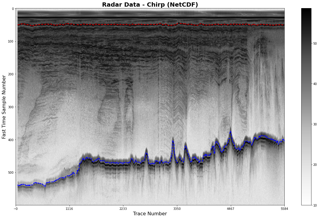
Plot the processed radargrams#
plt.rcParams['figure.figsize'] = [20,12] # set the size of the inline plot

fig1, ax1 = plt.subplots()
radar_im = ax1.imshow(chirpData[:600,:], cmap='Greys', vmin = 10, aspect='auto') # plot data (limit y-axis extent and colorscale)
ax1.plot(surf_pick,'r--', linewidth=2) # plot surface pick
ax1.plot(bed_pick, 'b--', linewidth=2) # plot bed pick
ax1.xaxis.set_major_locator(ticker.LinearLocator(6)) # set x-axis tick limits

ax1.set_title("Radar Data - Chirp (NetCDF)", fontsize = 20, fontweight = 'bold') # set title
ax1.set_xlabel("Trace Number", fontsize = 16) # set axis title
ax1.set_ylabel("Fast Time Sample Number", fontsize = 16) # set axis title
fig1.colorbar(radar_im, ax = ax1) # plot colorbar
<matplotlib.colorbar.Colorbar at 0x1e733870f10>
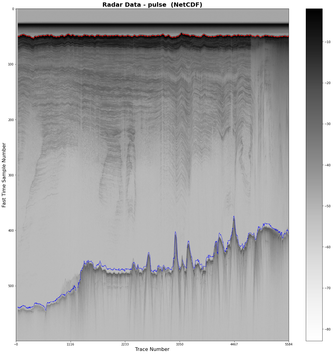
plt.rcParams['figure.figsize'] = [20,20] # set the size of the inline plot

fig2, ax2 = plt.subplots()
radar_im = ax2.imshow(pulseData[:600,:], cmap = 'Greys',  aspect='auto') # plot data (limit y-axis extent and colorscale)
ax2.plot(surf_pick,'r--', linewidth=2) # plot surface pick
ax2.plot(bed_pick, 'b--', linewidth=1) # plot bed pick
ax2.xaxis.set_major_locator(ticker.LinearLocator(6)) # set x-axis tick limits

ax2.set_title("Radar Data - pulse  (NetCDF)", fontsize = 20, fontweight = 'bold') # set title
ax2.set_xlabel("Trace Number", fontsize = 16) # set axis title
ax2.set_ylabel("Fast Time Sample Number", fontsize = 16) # set axis title
fig2.colorbar(radar_im, ax = ax2) # plot colorbar
<matplotlib.colorbar.Colorbar at 0x1e70ed627c0>
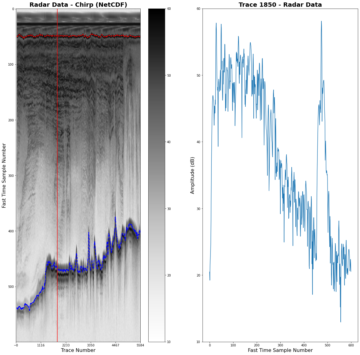
Plot amplitude of single trace from the radar data#
plt.rcParams['figure.figsize'] = [20,20] # set the size of the inline plot
fig2, (ax3, ax4) = plt.subplots(1, 2) # Specify how many plots you want

# first plot the radargram with specific trace marked as red vertical line
radar_im = ax3.imshow(chirpData[:600,:],cmap='Greys', vmin = 10, vmax = 60, aspect='auto') # plot data (limit y-axis extent and colorscale)
ax3.plot(surf_pick,'r--', linewidth=2) # plot surface pick
ax3.plot(bed_pick, 'b--', linewidth=2) # plot surface pick
ax3.xaxis.set_major_locator(ticker.LinearLocator(6)) # set x-axis tick limits
ax3.axvline(x=1850, color='r', linestyle='-') # plot position of trace in second plot
ax3.autoscale(enable=True, axis='x', tight=True) # tighten up x axis

ax3.set_title("Radar Data - Chirp (NetCDF)", fontsize = 20, fontweight = 'bold') # set title
ax3.set_xlabel("Trace Number", fontsize = 16)  # set axis title
ax3.set_ylabel("Fast Time Sample Number", fontsize = 16) # set axis title
fig2.colorbar(radar_im, ax = ax3) # plot colorbar

# then plot trace plot with amplitude and sampling window
ax4.plot(chirpData[:600,1850])
plt.title('Trace 1850 - Radar Data', fontsize = 20, fontweight = 'bold')  # set title
plt.xlabel('Fast Time Sample Number', fontsize = 16) # set axis title
plt.ylabel('Amplitude (dB)', fontsize = 16) # set axis title
plt.ylim([10,60]) # set limit of y-axis
plt.show()
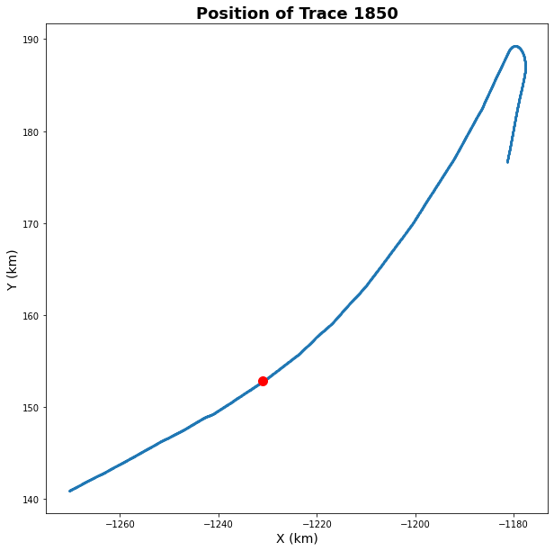
Plot geographic location of trace on map#
plt.rcParams['figure.figsize'] = [10,10] # Set the size of the inline plot

fig3, ax5 = plt.subplots(1,1)
plt.scatter(x_nc_km, y_nc_km, marker='o', s=1) # plot entire profile
plt.scatter(x_nc_km[1850], y_nc_km[1850], marker='o',color=['red'], s=100) # plot specific trace position as red dot

ax5.set_title("Position of Trace 1850", fontsize = 18, fontweight = 'bold') # set title
ax5.set_xlabel("X (km)", fontsize = 14) # set axis title
ax5.set_ylabel("Y (km)", fontsize = 14) # set axis title
Text(0, 0.5, 'Y (km)')
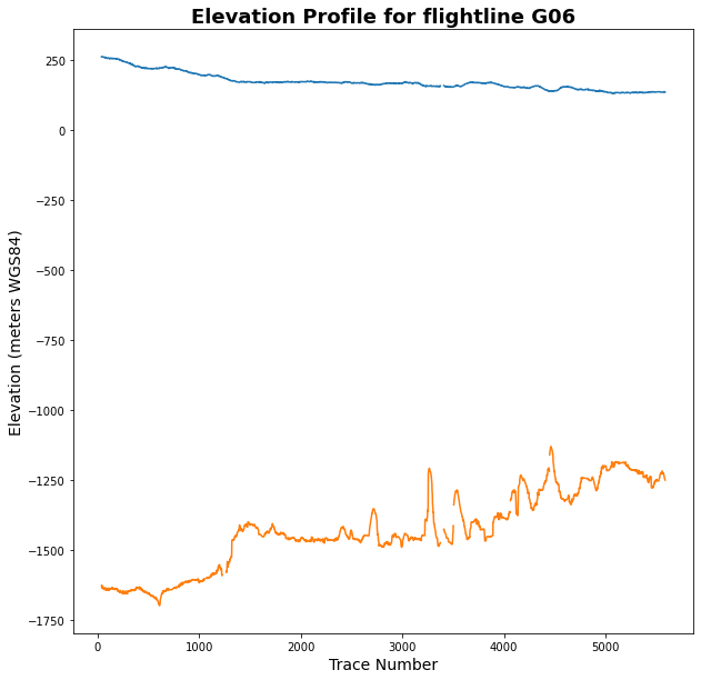
Plot surface and bed elevations along flightline#
plt.rcParams['figure.figsize'] = [10,10] # Set the size of the inline plot

fig4, ax6 = plt.subplots(1,1)
ax6.plot(traces_nc, surface_elevation) # plot surface elevation for entire profile
ax6.plot(traces_nc, bed_elevation) # plot bed elevation for entire profile

ax6.set_title("Elevation Profile for flightline G06", fontsize = 18, fontweight = 'bold') # set title
ax6.set_xlabel("Trace Number", fontsize = 14) # set axis title
ax6.set_ylabel("Elevation (meters WGS84)", fontsize = 14) # set axis title
Text(0, 0.5, 'Elevation (meters WGS84)')
Check the SEG-Y files#
Load the data for chirp and pulse#
Give here the path to where the desired files lives on your PC
segy_data_chirp = 'D:/British_Antarctic_Survey/data/GRADES_IMAGE_0607/segy/chirp/G06_chirp.segy'
segy_data_pulse = 'D:/British_Antarctic_Survey/data/GRADES_IMAGE_0607/segy/pulse/G06_pulse.segy'
Read the SEG-Ys#
The data is read using the _read_segy command from the obspy Python module
segy_chirp = _read_segy(segy_data_chirp, headonly=True)
segy_pulse = _read_segy(segy_data_pulse, headonly=True)
Inspect SEG-Y parameters#
It is possible to check the content of the SEG-Y bytes using very simple commands of the obspy package.
Some examples are given below for the chirp data (pulse is the same):
segy_chirp
5584 traces in the SEG Y structure.
header_segy = segy_chirp.binary_file_header
header_segy
Binary File Header:
	job_identification_number: 0
	line_number: 0
	reel_number: 0
	number_of_data_traces_per_ensemble: 0
	number_of_auxiliary_traces_per_ensemble: 0
	sample_interval_in_microseconds: 1000
	sample_interval_in_microseconds_of_original_field_recording: 0
	number_of_samples_per_data_trace: 1400
	number_of_samples_per_data_trace_for_original_field_recording: 0
	data_sample_format_code: 5
	ensemble_fold: 0
	trace_sorting_code: 0
	vertical_sum_code: 0
	sweep_frequency_at_start: 0
	sweep_frequency_at_end: 0
	sweep_length: 0
	sweep_type_code: 0
	trace_number_of_sweep_channel: 0
	sweep_trace_taper_length_in_ms_at_start: 0
	sweep_trace_taper_length_in_ms_at_end: 0
	taper_type: 0
	correlated_data_traces: 0
	binary_gain_recovered: 0
	amplitude_recovery_method: 0
	measurement_system: 1
	impulse_signal_polarity: 0
	vibratory_polarity_code: 0
	unassigned_1: b'\x00\x00\x00\x00\x00\x00\x00\x00\x00\x00\x00\x00\x00\x00\x00\x00\x00\x00\x00\x00\x00\x00\x00\x00\x00\x00\x00\x00\x00\x00\x00\x00\x00\x00\x00\x00\x00\x00\x00\x00\x00\x00\x00\x00\x00\x00\x00\x00\x00\x00\x00\x00\x00\x00\x00\x00\x00\x00\x00\x00\x00\x00\x00\x00\x00\x00\x00\x00\x00\x00\x00\x00\x00\x00\x00\x00\x00\x00\x00\x00\x00\x00\x00\x00\x00\x00\x00\x00\x00\x00\x00\x00\x00\x00\x00\x00\x00\x00\x00\x00\x00\x00\x00\x00\x00\x00\x00\x00\x00\x00\x00\x00\x00\x00\x00\x00\x00\x00\x00\x00\x00\x00\x00\x00\x00\x00\x00\x00\x00\x00\x00\x00\x00\x00\x00\x00\x00\x00\x00\x00\x00\x00\x00\x00\x00\x00\x00\x00\x00\x00\x00\x00\x00\x00\x00\x00\x00\x00\x00\x00\x00\x00\x00\x00\x00\x00\x00\x00\x00\x00\x00\x00\x00\x00\x00\x00\x00\x00\x00\x00\x00\x00\x00\x00\x00\x00\x00\x00\x00\x00\x00\x00\x00\x00\x00\x00\x00\x00\x00\x00\x00\x00\x00\x00\x00\x00\x00\x00\x00\x00\x00\x00\x00\x00\x00\x00\x00\x00\x00\x00\x00\x00\x00\x00\x00\x00\x00\x00\x00\x00\x00\x00\x00\x00\x00\x00\x00\x00\x00\x00'
	seg_y_format_revision_number: 100
	fixed_length_trace_flag: 1
	number_of_3200_byte_ext_file_header_records_following: 0
	unassigned_2: b'\x00\x00\x00\x00\x00\x00\x00\x00\x00\x00\x00\x00\x00\x00\x00\x00\x00\x00\x00\x00\x00\x00\x00\x00\x00\x00\x00\x00\x00\x00\x00\x00\x00\x00\x00\x00\x00\x00\x00\x00\x00\x00\x00\x00\x00\x00\x00\x00\x00\x00\x00\x00\x00\x00\x00\x00\x00\x00\x00\x00\x00\x00\x00\x00\x00\x00\x00\x00\x00\x00\x00\x00\x00\x00\x00\x00\x00\x00\x00\x00\x00\x00\x00\x00\x00\x00\x00\x00\x00\x00\x00\x00\x00\x00'
Read traces#
Obspy can also be used to read individual traces
traces = segy_chirp.traces
We can then have a look at the header of one specific trace, as follows:
trace_header = traces[1].header # for trace 1
trace_header
trace_sequence_number_within_line: 2
trace_sequence_number_within_segy_file: 2
original_field_record_number: 1185400
trace_number_within_the_original_field_record: 1
energy_source_point_number: 2
ensemble_number: 0
trace_number_within_the_ensemble: 0
trace_identification_code: 1
number_of_vertically_summed_traces_yielding_this_trace: 0
number_of_horizontally_stacked_traces_yielding_this_trace: 1
data_use: 0
distance_from_center_of_the_source_point_to_the_center_of_the_receiver_group: 0
receiver_group_elevation: 0
surface_elevation_at_source: 0
source_depth_below_surface: 0
datum_elevation_at_receiver_group: 0
datum_elevation_at_source: 0
water_depth_at_source: 0
water_depth_at_group: 0
scalar_to_be_applied_to_all_elevations_and_depths: 0
scalar_to_be_applied_to_all_coordinates: 0
source_coordinate_x: -1270327
source_coordinate_y: 140859
group_coordinate_x: 0
group_coordinate_y: 0
coordinate_units: 0
weathering_velocity: 0
subweathering_velocity: 0
uphole_time_at_source_in_ms: 0
uphole_time_at_group_in_ms: 0
source_static_correction_in_ms: 0
group_static_correction_in_ms: 0
total_static_applied_in_ms: 0
lag_time_A: 0
lag_time_B: 0
delay_recording_time: 0
mute_time_start_time_in_ms: 0
mute_time_end_time_in_ms: 0
number_of_samples_in_this_trace: 1400
sample_interval_in_ms_for_this_trace: 45
gain_type_of_field_instruments: 0
instrument_gain_constant: 0
instrument_early_or_initial_gain: 0
correlated: 0
sweep_frequency_at_start: 0
sweep_frequency_at_end: 0
sweep_length_in_ms: 0
sweep_type: 0
sweep_trace_taper_length_at_start_in_ms: 0
sweep_trace_taper_length_at_end_in_ms: 0
taper_type: 0
alias_filter_frequency: 0
alias_filter_slope: 0
notch_filter_frequency: 0
notch_filter_slope: 0
low_cut_frequency: 0
high_cut_frequency: 0
low_cut_slope: 0
high_cut_slope: 0
year_data_recorded: 2021
day_of_year: 273
hour_of_day: 3
minute_of_hour: 14
second_of_minute: 8
time_basis_code: 0
trace_weighting_factor: 0
geophone_group_number_of_roll_switch_position_one: 0
geophone_group_number_of_trace_number_one: 0
geophone_group_number_of_last_trace: 0
gap_size: 0
over_travel_associated_with_taper: 0
x_coordinate_of_ensemble_position_of_this_trace: 0
y_coordinate_of_ensemble_position_of_this_trace: 0
for_3d_poststack_data_this_field_is_for_in_line_number: 0
for_3d_poststack_data_this_field_is_for_cross_line_number: 0
shotpoint_number: 0
scalar_to_be_applied_to_the_shotpoint_number: 0
trace_value_measurement_unit: 0
transduction_constant_mantissa: 0
transduction_constant_exponent: 0
transduction_units: 0
device_trace_identifier: 0
scalar_to_be_applied_to_times: 0
source_type_orientation: 0
source_energy_direction_mantissa: 0
source_energy_direction_exponent: 0
source_measurement_mantissa: 0
source_measurement_exponent: 0
source_measurement_unit: 0
We can also check the amount of traces in the file (x-axis):
sgy_traces_len = len(segy_chirp.traces)
sgy_traces_len
5584
And check the length of the sampling window (y-axis)
sgy_samples_len = traces[1].header.number_of_samples_in_this_trace
sgy_samples_len
1400
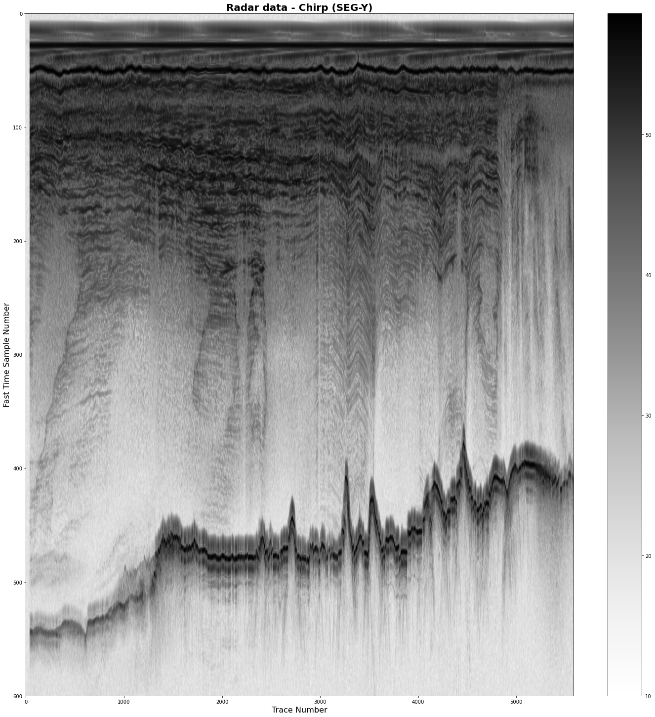
Plot the processed radargrams#
We first need to concatenate all traces from the SEG-Y into one array and calculate the log of data
data_chirp = np.stack(t.data for t in segy_chirp.traces) # concatenate
data_chirp = 10*np.log10(data_chirp) # convert the data from power to decibels using log of data
data_pulse = np.stack(t.data for t in segy_pulse.traces) # concatenate
data_pulse = 10*np.log10(data_pulse) # convert the data from power to decibels using log of data
Now we can plot them:
plt.rcParams["figure.figsize"] = (20,20) # set the size of the inline plot

fig4, ax6 = plt.subplots()
plt.imshow(data_chirp.T, cmap='Greys', vmin = 10, aspect='auto') # plot data (limit colorscale extent)
plt.title('Radar data - Chirp (SEG-Y)', fontsize = 20, fontweight = 'bold') # set title
plt.colorbar() # plot colorbar
plt.tight_layout() # tighten up x axis
plt.ylim([600,0]) # set y-axis limits
ax5.set_xlabel("Trace Number", fontsize = 16) # set axis title
ax5.set_ylabel("Fast Time Sample Number", fontsize = 16) # set axis title
Text(143.5, 0.5, 'Fast Time Sample Number')
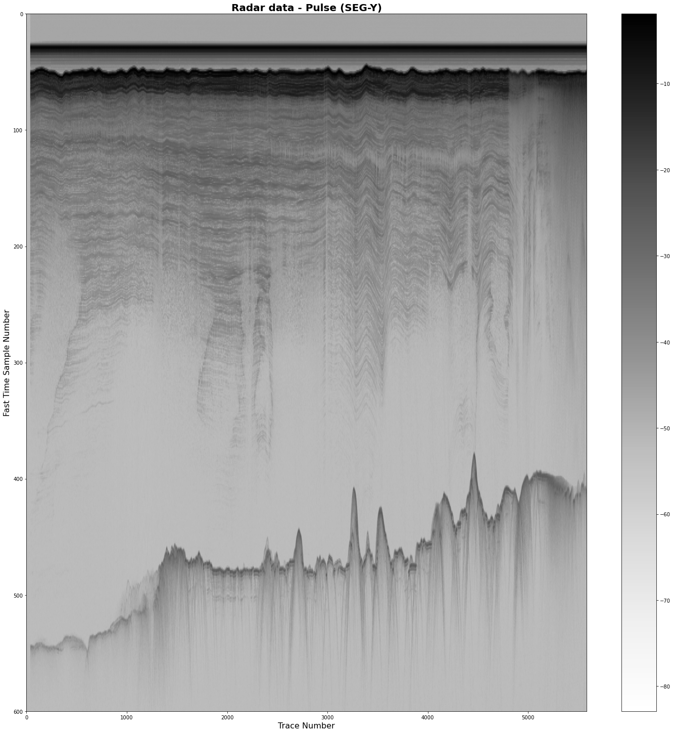
plt.rcParams["figure.figsize"] = (20,20) # set the size of the inline plot

fig5, ax7 = plt.subplots()
plt.imshow(data_pulse.T, cmap='Greys', aspect='auto') # plot data (limit colorscale extent)
plt.title('Radar data - Pulse (SEG-Y)', fontsize = 20, fontweight = 'bold') # set title
plt.colorbar() # plot colorbar
plt.tight_layout() # tighten up x axis
plt.ylim([600,0]) # set y-axis limits
ax6.set_xlabel("Trace Number", fontsize = 16) # set axis title
ax6.set_ylabel("Fast Time Sample Number", fontsize = 16) # set axis title
Text(143.5, 0.5, 'Fast Time Sample Number')