Checking Airborne Magnetics data#
Author: Alice Fremand (@almand)
Date: 12/11/2021
Aim#
The goal of this tutorial is to easily check the airborne gravity data provided in XYZ format.
Virtual environment#
For the code to run, it is important to install the correct dependancies and libraries. In particular the following libraries are crucial for the code to be run:
pandas module to check CSV and text data in python
geopandas module to check data geospatially in python
To set up the virtual environment with Conda:#
>conda create -n aerogeophysics_env
>conda activate aerogeophysics_env
>conda config --env --add channels conda-forge
>conda config --env --set channel_priority strict
>conda install python=3 geopandas
To set up the virtual environment on UNIX:#
Load your python module:
module load python/conda3
Then in the folder where you have your code, you need to launch:
python3 -m venv aerogeophysics_env
It will create a folder with all the environment for python. To activate the virtual environment you need to lauch it:
source aerogeophysics_env/bin/activate.csh
You need to make sure that [aerogeophysics_env] appears before your name on the machine. That means that you are using the virtual environment Then you need to upgrade pip which is the command that install the packages
python3 -m pip install --upgrade pip
And install the other libraries
python3 -m pip install geopandas
In this tutorial, the virtual environment is already set up. The list of the current libraries loaded is given in the list below.
pip list
Package                       Version
----------------------------- -------------------
alabaster                     0.7.12
anyio                         3.3.4
argon2-cffi                   21.1.0
async-generator               1.10
attrs                         21.2.0
Babel                         2.9.1
backcall                      0.2.0
backports.functools-lru-cache 1.6.4
beautifulsoup4                4.10.0
bleach                        4.1.0
brotlipy                      0.7.0
certifi                       2021.10.8
cffi                          1.15.0
cftime                        1.5.1.1
chardet                       4.0.0
charset-normalizer            2.0.0
click                         7.1.2
click-completion              0.5.2
click-log                     0.3.2
click-plugins                 1.1.1
cligj                         0.7.1
cloudpickle                   1.6.0
colorama                      0.4.4
cryptography                  35.0.0
cycler                        0.10.0
dataclasses                   0.8
decorator                     5.0.9Note: you may need to restart the kernel to use updated packages.
defusedxml                    0.7.1

docutils                      0.16
entrypoints                   0.3
Fiona                         1.8.18
future                        0.18.2
GDAL                          3.1.4
geopandas                     0.9.0
gitdb                         4.0.9
GitPython                     3.1.24
greenlet                      1.1.2
idna                          3.1
imagesize                     1.3.0
importlib-metadata            4.8.2
importlib-resources           3.3.1
ipykernel                     5.5.5
ipython                       7.23.1
ipython-genutils              0.2.0
ipywidgets                    7.6.5
jedi                          0.18.0
Jinja2                        3.0.3
jsonschema                    3.2.0
jupyter                       1.0.0
jupyter-book                  0.12.0
jupyter-cache                 0.4.3
jupyter-client                6.1.12
jupyter-console               6.4.0
jupyter-core                  4.7.1
jupyter-server                1.11.2
jupyter-server-mathjax        0.2.3
jupyter-sphinx                0.3.2
jupyterlab-pygments           0.1.2
jupyterlab-widgets            1.0.2
jupytext                      1.11.5
kiwisolver                    1.3.2
latexcodec                    2.0.1
linkify-it-py                 1.0.2
lxml                          4.6.4
markdown-it-py                1.1.0
MarkupSafe                    2.0.1
matplotlib                    3.4.3
matplotlib-inline             0.1.2
mdit-py-plugins               0.2.8
mistune                       0.8.4
munch                         2.5.0
myst-nb                       0.13.1
myst-parser                   0.15.2
nbclient                      0.5.5
nbconvert                     6.2.0
nbdime                        3.1.1
nbformat                      5.1.3
nest-asyncio                  1.5.1
netCDF4                       1.5.7
notebook                      6.4.5
numpy                         1.20.3
obspy                         1.2.2
olefile                       0.46
packaging                     21.2
pandas                        1.2.4
pandocfilters                 1.5.0
parso                         0.8.2
pickleshare                   0.7.5
Pillow                        8.3.1
pip                           21.1.2
prometheus-client             0.12.0
prompt-toolkit                3.0.18
pybtex                        0.24.0
pybtex-docutils               1.0.1
pycparser                     2.21
pydata-sphinx-theme           0.6.3
Pygments                      2.9.0
pyOpenSSL                     21.0.0
pyparsing                     2.4.7
pyproj                        3.1.0
PyQt5                         5.12.3
PyQt5-sip                     4.19.18
PyQtChart                     5.12
PyQtWebEngine                 5.12.1
pyrsistent                    0.18.0
PySocks                       1.7.1
python-dateutil               2.8.1
pytz                          2021.1
pywin32                       300
pywinpty                      1.1.4
PyYAML                        6.0
pyzmq                         22.1.0
qtconsole                     5.1.1
QtPy                          1.11.2
requests                      2.26.0
Rtree                         0.9.7
scipy                         1.6.3
Send2Trash                    1.8.0
setuptools                    49.6.0.post20210108
Shapely                       1.7.1
shellingham                   1.4.0
six                           1.16.0
smmap                         3.0.5
sniffio                       1.2.0
snowballstemmer               2.1.0
soupsieve                     2.3
Sphinx                        4.3.0
sphinx-book-theme             0.1.6
sphinx-comments               0.0.3
sphinx-copybutton             0.4.0
sphinx-external-toc           0.2.3
sphinx-jupyterbook-latex      0.4.5
sphinx-multitoc-numbering     0.1.3
sphinx-panels                 0.6.0
sphinx-thebe                  0.0.10
sphinx-togglebutton           0.2.3
sphinxcontrib-applehelp       1.0.2
sphinxcontrib-bibtex          2.2.1
sphinxcontrib-devhelp         1.0.2
sphinxcontrib-htmlhelp        2.0.0
sphinxcontrib-jsmath          1.0.1
sphinxcontrib-qthelp          1.0.3
sphinxcontrib-serializinghtml 1.1.5
spyder-kernels                1.10.2
SQLAlchemy                    1.4.26
terminado                     0.12.1
testpath                      0.5.0
toml                          0.10.2
tornado                       6.1
traitlets                     5.0.5
typing-extensions             3.10.0.2
uc-micro-py                   1.0.1
urllib3                       1.26.7
wcwidth                       0.2.5
webencodings                  0.5.1
websocket-client              0.57.0
wheel                         0.36.2
widgetsnbextension            3.5.2
win-inet-pton                 1.1.0
wincertstore                  0.2
zipp                          3.6.0
Load the relevant modules#
import os
import glob
import pandas as pd
import numpy as np
import geopandas as gpd
import os
import matplotlib.pyplot as plt
#Specific module to plot the graph in the Jupyter Notebook
%matplotlib inline
Checking the XYZ files#
Example given for GRADES-IMAGE data.
Data available for download here: Ferraccioli, F., & Jordan, T. (2020). Airborne magnetic data covering the Evans, and Rutford Ice Streams, and ice rises in the Ronne Ice Shelf (2006/07) (Version 1.0) [Data set]. UK Polar Data Centre, Natural Environment Research Council, UK Research & Innovation. https://doi.org/10.5285/7504BE9B-93BA-44AF-A17F-00C84554B819
Reading the XYZ data#
aeromag_data = 'E:/UKPDC/JupyterExample/AGAP_Mag.XYZ'
The XYZ data are composed of a large header and empty rows at the top. To read the file, it is recommended to remove these empty rows. The goal is to keep the 5th row which corresponds to the header but remove all the other ten first rows, we can specify these rows like this:
skiprow= list(range(0,11))
skiprow.remove(5)
skiprow
[0, 1, 2, 3, 4, 6, 7, 8, 9, 10]
Then, we can use pandas to read the data. The data are separated by a space, we can specify the separator by using the sep parameter, we will use `skiprow
file = pd.read_csv(aeromag_data, skiprows=skiprow, sep= ' +', engine='python' )
file.head()
| / | Flight_ID | Line_no | Lon | Lat | x | y | Height_WGS1984 | Date | Time | ... | BCorr_AGAP_NS | BCorr_AGAP_S | BCorr_AGAP_SP | BCorr_Applied | MagBRTC | ACorr | SCorr | MagF | MagL | MagML | |
|---|---|---|---|---|---|---|---|---|---|---|---|---|---|---|---|---|---|---|---|---|---|
| 0 | CTAM1 | 5.0 | 154.333738 | -83.785881 | 2673830.187189 | 1076723.517935 | 3150.4 | 2008/12/08 | 03:30:04.00 | * | ... | * | * | * | * | * | * | * | * | * | NaN |
| 1 | CTAM1 | 5.0 | 154.332907 | -83.786293 | 2673783.220184 | 1076719.879693 | 3151.2 | 2008/12/08 | 03:30:05.00 | 59475.32 | ... | * | -15.15 | 15.15 | -148.65 | * | * | -148.65 | -148.65 | -148.65 | NaN |
| 2 | CTAM1 | 5.0 | 154.332099 | -83.786706 | 2673736.205959 | 1076715.921844 | 3152.1 | 2008/12/08 | 03:30:06.00 | 59475.17 | ... | * | -15.14 | 15.14 | -148.47 | * | * | -148.47 | -148.47 | -148.47 | NaN |
| 3 | CTAM1 | 5.0 | 154.331331 | -83.787120 | 2673689.204893 | 1076711.467081 | 3153.4 | 2008/12/08 | 03:30:07.00 | 59475.19 | ... | * | -15.13 | 15.13 | -148.28 | * | * | -148.28 | -148.28 | -148.28 | NaN |
| 4 | CTAM1 | 5.0 | 154.330608 | -83.787535 | 2673642.281478 | 1076706.469544 | 3154.9 | 2008/12/08 | 03:30:08.00 | 59475.19 | ... | * | -15.12 | 15.12 | -148.08 | * | * | -148.08 | -148.08 | -148.08 | NaN |
5 rows × 26 columns
As we can see, the first column is filled with 0, so we might want to remove it:
column_names = file.columns.tolist()
column_names.remove('/')
column_names.append('toDelete')
file.columns = column_names
file = file.drop(columns='toDelete')
file.head()
| Flight_ID | Line_no | Lon | Lat | x | y | Height_WGS1984 | Date | Time | MagR | ... | BCorr_AGAP_NS | BCorr_AGAP_S | BCorr_AGAP_SP | BCorr_Applied | MagBRTC | ACorr | SCorr | MagF | MagL | MagML | |
|---|---|---|---|---|---|---|---|---|---|---|---|---|---|---|---|---|---|---|---|---|---|
| 0 | CTAM1 | 5.0 | 154.333738 | -83.785881 | 2673830.187189 | 1076723.517935 | 3150.4 | 2008/12/08 | 03:30:04.00 | * | ... | * | * | * | * | * | * | * | * | * | * |
| 1 | CTAM1 | 5.0 | 154.332907 | -83.786293 | 2673783.220184 | 1076719.879693 | 3151.2 | 2008/12/08 | 03:30:05.00 | 59475.32 | ... | * | * | -15.15 | 15.15 | -148.65 | * | * | -148.65 | -148.65 | -148.65 |
| 2 | CTAM1 | 5.0 | 154.332099 | -83.786706 | 2673736.205959 | 1076715.921844 | 3152.1 | 2008/12/08 | 03:30:06.00 | 59475.17 | ... | * | * | -15.14 | 15.14 | -148.47 | * | * | -148.47 | -148.47 | -148.47 |
| 3 | CTAM1 | 5.0 | 154.331331 | -83.787120 | 2673689.204893 | 1076711.467081 | 3153.4 | 2008/12/08 | 03:30:07.00 | 59475.19 | ... | * | * | -15.13 | 15.13 | -148.28 | * | * | -148.28 | -148.28 | -148.28 |
| 4 | CTAM1 | 5.0 | 154.330608 | -83.787535 | 2673642.281478 | 1076706.469544 | 3154.9 | 2008/12/08 | 03:30:08.00 | 59475.19 | ... | * | * | -15.12 | 15.12 | -148.08 | * | * | -148.08 | -148.08 | -148.08 |
5 rows × 25 columns
As you can see, a number of values are given a star for non value data. In this analysis, we are only interested n the longitude, latitude and magnetics anomaly. We will thus select these specific parameters.
Selecting the variables#
longitude = [variable for variable in file.columns.tolist() if (variable.startswith('Lon'))][0]
latitude = [variable for variable in file.columns.tolist() if (variable.startswith('Lat'))][0]
mag = [variable for variable in file.columns.tolist() if (variable.startswith('MagF'))][0]
file = file[[longitude,latitude, mag]]
file = file.replace('*', np.nan)
file = file.dropna()
file[longitude] = file[longitude].astype(float) #To make sure lat and Lon are float
file[latitude] = file[latitude].astype(float)
file[mag] = file[mag].astype(float)
file.head()
| Lon | Lat | MagF | |
|---|---|---|---|
| 1 | 154.332907 | -83.786293 | -148.65 |
| 2 | 154.332099 | -83.786706 | -148.47 |
| 3 | 154.331331 | -83.787120 | -148.28 |
| 4 | 154.330608 | -83.787535 | -148.08 |
| 5 | 154.329925 | -83.787950 | -147.89 |
We can also get some specific parameters:
ID = aeromag_data.split('/')[-1].strip('.XYZ')
survey = aeromag_data.split('/')[3]
print('''ID: %s
Survey: %s
Name of magnetic variable: %s
Name of longitude variable: %s
Name of latitude variable: %s''' %(ID, survey, mag, longitude, latitude))
ID: AGAP_Mag
Survey: AGAP_Mag.XYZ
Name of magnetic variable: MagF
Name of longitude variable: Lon
Name of latitude variable: Lat
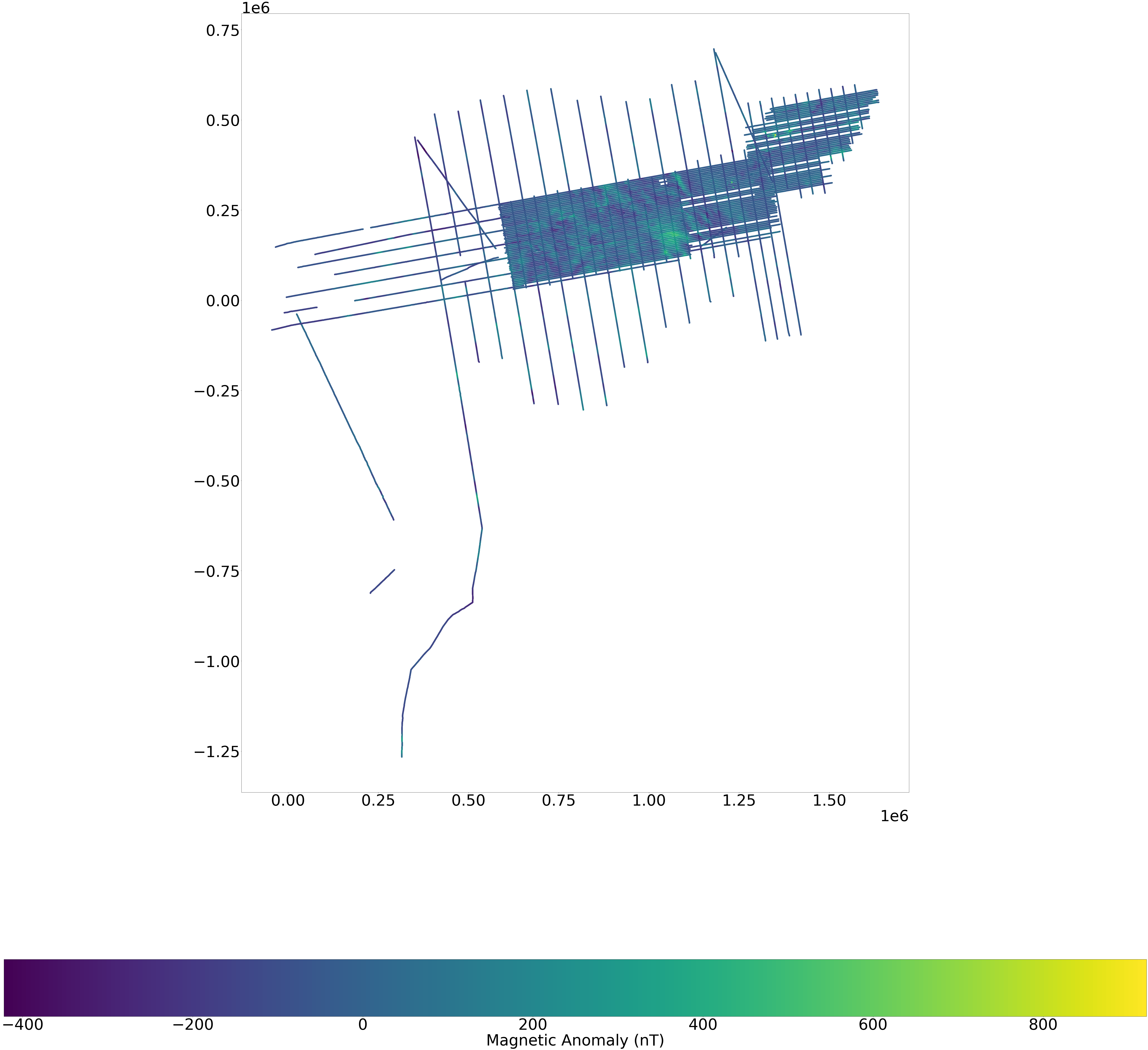
Have a look at the data geospatially#
We can easily convert the data to spatial objects using geopandas. The geopandas module is used to convert the data to a geodataframe. It will convert the latitude/longitude to points.
To do that, you will need to identify the specific header used for longitude and latitude in the CSV file.
gdf = gpd.GeoDataFrame(file, geometry=gpd.points_from_xy(file[longitude], file[latitude]))
We can check the conversion:
gdf.head()
| Lon | Lat | MagF | geometry | |
|---|---|---|---|---|
| 1 | 154.332907 | -83.786293 | -148.65 | POINT (154.33291 -83.78629) |
| 2 | 154.332099 | -83.786706 | -148.47 | POINT (154.33210 -83.78671) |
| 3 | 154.331331 | -83.787120 | -148.28 | POINT (154.33133 -83.78712) |
| 4 | 154.330608 | -83.787535 | -148.08 | POINT (154.33061 -83.78754) |
| 5 | 154.329925 | -83.787950 | -147.89 | POINT (154.32993 -83.78795) |
Setting up the coordinate system#
It is important to then set the coordinate system. Here the WGS84 coordinate system is used, it corresponds to the EPSG: 4326.
gdf = gdf.set_crs("EPSG:4326")
With geopandas, it is also possible to convert the data to another coordinate system and project it. You just need to know the EPSG ID of the output coordinate system. Here is how to convert the data to the Polar Antarctic stereographic geographic system (https://epsg.io/3031).
gdf = gdf.to_crs("EPSG:3031")
Plotting the data#
plt.rcParams["figure.figsize"] = (100,100)
plt.rcParams.update({'font.size': 75})
fig, ax = plt.subplots(1, 1)
fig=plt.figure(figsize=(100,100), dpi= 100, facecolor='w', edgecolor='k')
gdf.plot(column=mag, ax=ax, legend=True, legend_kwds={'label': "Magnetic Anomaly (nT)",'orientation': "horizontal" })
<AxesSubplot:>
<Figure size 10000x10000 with 0 Axes>
Calculate statistics about the data#
Size of the dataset#
size = round(os.path.getsize(aeromag_data)/1e+6)
print('size: %s MB' %size)
size: 513 MB
Magnetics anomaly statistics#
mean_mag=round(file[mag].mean())
max_mag=round(file[mag].max())
latlong_max_mag=(file[longitude][file[mag].idxmax()],file[latitude][file[mag].idxmax()])
min_mag=round(file[mag].min())
latlong_min_mag=(file[longitude][file[mag].idxmin()],file[latitude][file[mag].idxmin()])

print('''
Mean magnetic anomaly: %s nT
Max magnetic anomaly: %s nT
Longitude and latitude of maximum magnetic anomaly: %s
Minimum magnetic anomaly: %s nT
Longitude/Latitude of minimum magnetic anomaly: %s''' %(mean_mag, max_mag, latlong_max_mag, min_mag, latlong_min_mag))
Mean magnetic anomaly: -12 nT
Max magnetic anomaly: 921 nT
Longitude and latitude of maximum magnetic anomaly: (71.247489, -76.942731)
Minimum magnetic anomaly: -422 nT
Longitude/Latitude of minimum magnetic anomaly: (41.734519, -84.813545)
Calculate distance along the profile#
file['distance'] = gdf.distance(gdf.shift(1))
distance_total=round(sum(file.distance[file.distance<15000])/1000)
print('Dstance along the profile: %s km' %distance_total)
Dstance along the profile: 73676 km
Calculate number of points#
nb_points= len(file)
print('Number of points: %s' %nb_points)
Number of points: 1109941
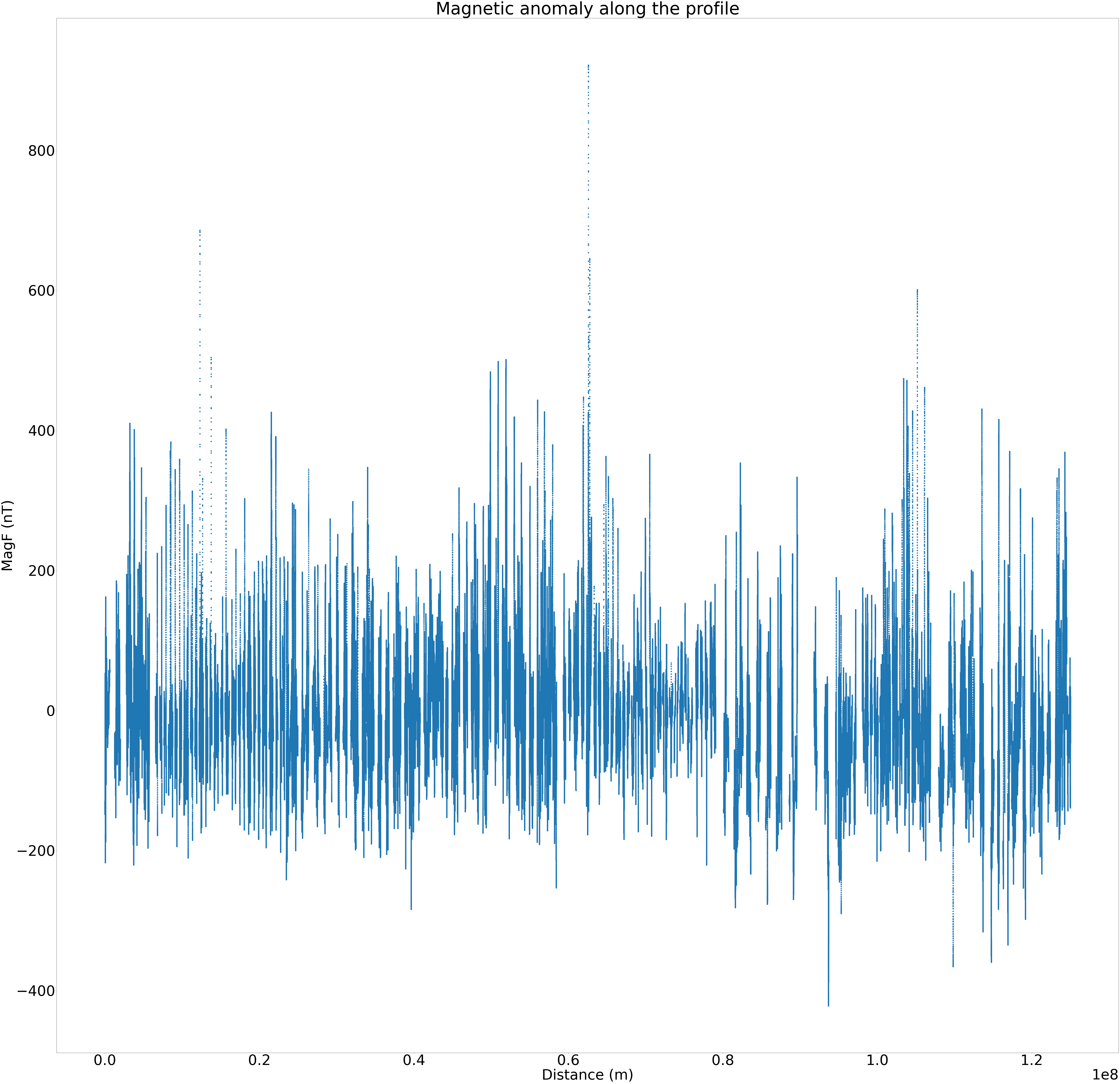
Looking at the magnetics anomaly along the profile#
file['distance'] = file['distance'].cumsum() #To have the cumulative sum of the distance
plt.scatter(file.distance, file[mag])
plt.xlabel('Distance (m)')
plt.ylabel('%s (nT)' %mag)
plt.title('Magnetic anomaly along the profile')
Text(0.5, 1.0, 'Magnetic anomaly along the profile')